Global Healthy & Sustainable City Indicators software
GHSCI
Overview
The Global Healthy and Sustainable City Indicators (GHSCI, or global-indicators) software is an open-source tool for measuring, monitoring and reporting on policy and spatial urban indicators for healthy, sustainable cities worldwide using open or custom data. Designed to support participation in the Global Observatory of Healthy and Sustainable Cities’ 1000 city challenge, it can be run as code or as an app in your web browser.
The software can be configured to support comparisons within- and between-cities and across time, benchmarking, analysis and monitoring of local policies, tracking progress, and inform interventions towards achieving healthy, equitable and sustainable cities (Figure 1). It also supports generating resources including maps, figures and reports in multiple languages, so these can be made accessible for use by local communities and stakeholders as a source of evidence to advocate for change.
Figure 1. The GHSCI tool can be used to create and report on policy and spatial indicators for cities around the world from your web browser, or optionally as code, a Jupyter notebook, or from command line
What does this do?
The software can be configured to calculate and report on policy and spatial indicators for healthy and sustainable cities in diverse contexts globally. The core set of spatial indicators are calculated for point locations, a small area grid (e.g. 100m), and overall city estimates. Optionally, indicators can also be calculated for custom areas, like administrative boundaries or specific neighbourhoods of interest. In addition CSV files containing indicators for area summaries and the overall city are also generated, omitting geometry. Metadata and data dictionaries are generated to accompany the data, along with reports in multiple languages.
The default core set of spatial urban indicators calculated includes:
Urban area in square kilometres
Population density (persons per square kilometre)
Street connectivity (intersections per square kilometre)
Access to destinations within 500 meters:
a supermarket
a convenience store
a public transport stop (any; or optionally, regularly serviced)
a public open space (e.g. park or square; any, or larger than 1.5 hectares)
A score for access to a range of daily living amenities
The resulting city-specific resources can be used to provide evidence to support policy makers and planners to strengthen urban policy, target interventions within cities, compare performance across cities, and when measured across time can be used to monitor progress towards achieving urban design goals for reducing inequities. Moreover, they provide a rich source of data for those advocating for disadvantaged and vulnerable community populations.
Generated outputs include:
Summary of configuration parameters used for analysis (.yml file)
Processing log detailing the analyses undertaken (.txt file)
Geopackage of indicator results and spatial features including points and areas of interest and pedestrian network (.gpkg)
CSV files for indicator results (.csv)
Data dictionaries (.csv and .xlsx files)
ISO19115 metadata (.xml and .yml files)
Analysis report (pdf)
Policy and spatial indicator report, optionally in multiple languages (.pdf)
Figures and maps, optionally in multiple languages (.jpg)
The software is designed to be used by local experts as part of multi-disciplinary teams participating in the 1000 Cities Challenge; but anyone (e.g. students, enthusiasts) can use the open source software.
How to set up and get started
Usage in brief
The Global Healthy and Sustainable Cities Indicators (GHSCI) tool can be run in a web browser or as Python code (e.g. in Jupyter Lab). Once the software environment has been retrieved and is running, analysis for a particular city proceeds in four steps:
Compare results (e.g. impact of hypothetical scenarios and sensitivity analyses, benchmarking between cities or regions of interest, monitoring change across time)
A fully configured example study region is provided along with data for users to familiarise themselves with the workflow and the possibilities of the generated resources. The instructions below will describe how to perform the analysis, and how to access, run and modify the provided example Jupyter notebook to perform analyses for your own study regions.
Software set up
Download and unzip the GHSCI software to a desired project directory on your computer
Install and run Docker Desktop according to the guidelines for your operating system of choice
Run the GHSCI software by opening the project directory where you extracted the software using a command line interface (e.g. Terminal on Windows, Terminal on MacOS, or Bash on Linux):
on Windows open the folder in Terminal or cmd.exe and enter ‘.\global-indicators.bat’
on MacOS/Linux in bash, enter ‘bash ./global-indicators.sh’
Linux users may need to prefix this with ‘sudo’ for elevated permissions when launching Docker containers (read more here)
This will retrieve the computational environment and launch the Global Healthy and Sustainable City Indicators (GHSCI) software, along with a PostGIS spatial database that is used for processing and data management. Once launched, instructions will be displayed (Figure 2).
Figure 2. With Docker Desktop installed and running, run the global-indicators command to initialise the software environment and view usage instructions
Running the software
The software can be used to configure study regions, conduct analysis, generate resources and compare results in four ways, depending on preference:
Web app
To launch the app in your web browser, type ghsci and open the displayed URL in your web browser
Jupyter Lab
To use a Jupyter Notebook, type lab, open the displayed URL in your web browser and double click to select the example notebook example.ipynb from the left-hand side browser pane
Command line
The basic shortcut commands configure, analysis, generate and compare can be run at the commandline in conjunction with a codename referring to your study region
Python
Optionally, the process can be run in Python, for example:
import ghsci
# set a codename for your city; here is the codename for the provided example
codename = 'example_ES_Las_Palmas_2023'

# Initialise configuration file for your region
r = ghsci.Region(codename)

# Now, you need to source and download data, documenting metadata and file paths in the configuration file generated in the process/configuration/regions directory
# Once that is completed, you can proceed:
r.analysis()
r.generate()

# if you've analysed and generated results for other study regions, you can compare the main results
r.compare('another_previously_processed_codename')

# if for some reason you want to drop the database for your study region to start again:
r.drop()

# You will be asked if you really want to do this!  It requires entering "ghscic" to confirm
# This doesn't remove any generated files or folders - you'll have to remove those yourself, if you want to.
Example analysis
An example region fully configured with downloaded data has been provided for Las Palmas de Gran Canaria in Spain with a target year of 2023. See the file process/configuration/regions/example_ES_Las_Palmas_2023.yml to view configured settings and paths to data provided for this example city. This section will demonstrate how to perform an analysis of this region, using the GHSCI graphical user interface app in your web browser. The same example has also been provided as a Jupyter notebook (example.ipynb), that may be selected and opened from within Jupyter Lab.
From the launched software prompt, type ghsci to start the web app and click the displayed link to open a web browser at http://localhost:8080.
Configuration
The Global Healthy and Sustainable City Indicators app opens to a tab for selecting or creating a new study region (Figure 3). We can see that the city of Las Palmas de Gran Canaria, Spain has been Configured but hasn’t yet had analysis perormed or resources generated. Once two configured regions have had their resources generated, they can be compared. Additionally, the results of a completed policy checklist can be summarised and queried.
Figure 3. Create, search and view summary details for your study regions using the GHSCI web app interface before performing analysis, generating resources, running comparisons, or querying the results of a policy audit.
Analysis
To run the example, click to select ‘example_ES_Las_Palmas_2023’ in the table, head to the Analysis tab and click the button. While analysis is being conducted, progress will be summarised in the terminal. This may take a few minutes to complete (Figure 4).
Figure 4. Performing analysis and generating resources will run code in the terminal window; view the outputs of these steps as they run to receive more information on what to do next.
Once completed, if you return to the ‘Study regions’ tab the study region summary will have the Analysed check box ticked and if you click to select the example in the table it will display the configured study region boundary on the map (Figure 5).
Figure 5. The study region boundary can be visualised on a map.
Click the study region to view a popup summary of the core set of indicators calculated (spatial distribution data will be generated shortly, and directions for producing an interactive map are provided in the example Jupyter notebook).
Generate
To generate the range of resources listed above, with the example city selected navigate to the Generate tab and click the Generate resources button. A series of outputs generated will be reported in the terminal window (Figure 6), and can be located in the study region’s data output folder (Figure 7).
Figure 6. The list of generated resources is summarised in the terminal window, while a summary of core indicators for the region can be viewed on the interactive map.
Figure 7. The list of generated folders and files following analysis and generating resources for a city.
A log file will be generated in the study region folder that can assist with debugging if things go wrong, or otherwise verifying the process has been successful and let you see some of the details of how things are processed. For the example city, this file is __Las Palmas de Gran Canaria__example_ES_Las_Palmas_2023_processing_log.txt.
The file _parameters.yml contains a record of your project, region and data configurations that gave rise to the generated outputs. Spatial features used in analysis as well as grid and overall city summaries are saved within a geopackage file, and CSV files of final summary results are provided too.
The PDF reports (Figures 8 and 9) are located within the folder _web reports, while the maps and images generated for use in that report (Figure 10) are located in the figures folder.
Figure 8. PDF reports in English and Spanish for Las Palmas.
Figure 9. Example page from the Spanish PDF policy and spatial indicators report for Las Palmas (policy results have not been completed and are are included for illustration purposes only).
Figure 10. Generated plot and map figures from the analysis of Las Palmas, with annotations in English and Spanish.
Compare
You can use the Compare function to
evaluate the overall impact of parameters and data used (sensitivity analyses)
compare results of different cities (benchmarking)
compare results for the same study region across time (monitoring)
evaluate the impact of hypothetical scenarios or interventions through analysis of modified data to represent these
The following section provides an example of how the compare functionality of the GHSCI tool can be used to evaluate aspects such as those listed above.
Sensitivity analyses
Sensitivity analyses can be performed to evaluate how methodological decisions, such as the way in which a study region boundary has been defined, can influence spatial urban indicator results. In our example, we used an empirical definition of our study region’s urban area. This is important, because administrative boundaries are often broader expanses that may include industrial or rural areas with low or no usual resident population that may impede comparability if we sought to benchmark our results with another city; an empirical or external definition for what is ‘urban’ can help our results be more comparable. The impact of this choice should be understood however, and depending on context and the needs of those who would use the indicator data and estimates produced, customisation of boundary definition may be required.
To perform an example sensitivity analysis evaluating the impact of restricting analysis using an empirically identified urban area (Figure 11):
take a copy of the ‘example_ES_Las_Palmas_2023.yml’ file and save it as ES_Las_Palmas_2023_test_not_urbanx.
Open this file in a text editor and
modify the entry under study_region_boundary reading ghsl_urban_intersection: true to ghsl_urban_intersection: false
modify the value of the parameter entry for ‘notes’ (line 57) to read “This supplementary configuration file for the broader administrative boundary region of Las Palma allows the impact of restricting analysis to the urban region (as per the main example) to be evaluated.”
now, exit the application (click the button in the top right hand corner) and restart the application
select the new region and perform the analysis and generate resources steps
select the example_ES_Las_Palmas_2023 study region and navigate to the Compare tab
select the ES_Las_Palmas_2023_test_not_urbanx region from the comparison drop down menu and click Compare study regions to generate a comparison CSV in the example study region’s output folder (process\data\_study_region_outputs\example_ES_Las_Palmas_2023) and display a table with side-by-side comparison of the overall region statistics and indicator estimates in the app window:
Figure 11. A summary of core indicators can be generated; values are rounded for display purposes, but the comparison analysis also generates a dated CSV file located in the output folder of the selected reference region with un-rounded values.
This technique can be used to summarise the overall impacts of a range of choices and assumptions relating to the choice of data and parameters to be used in analysis. Users are encouraged to also examine the generated spatial indicator layers using a Desktop GIS software like QGIS to evaluate the appropriateness of data inputs and the results arising from how study regions have been configured.
Analogously, the same technique could be applied to compare the change in results when using data that has been modified to represent some kind of scenario or intervention and evaluate its impact on relevant urban indicators.
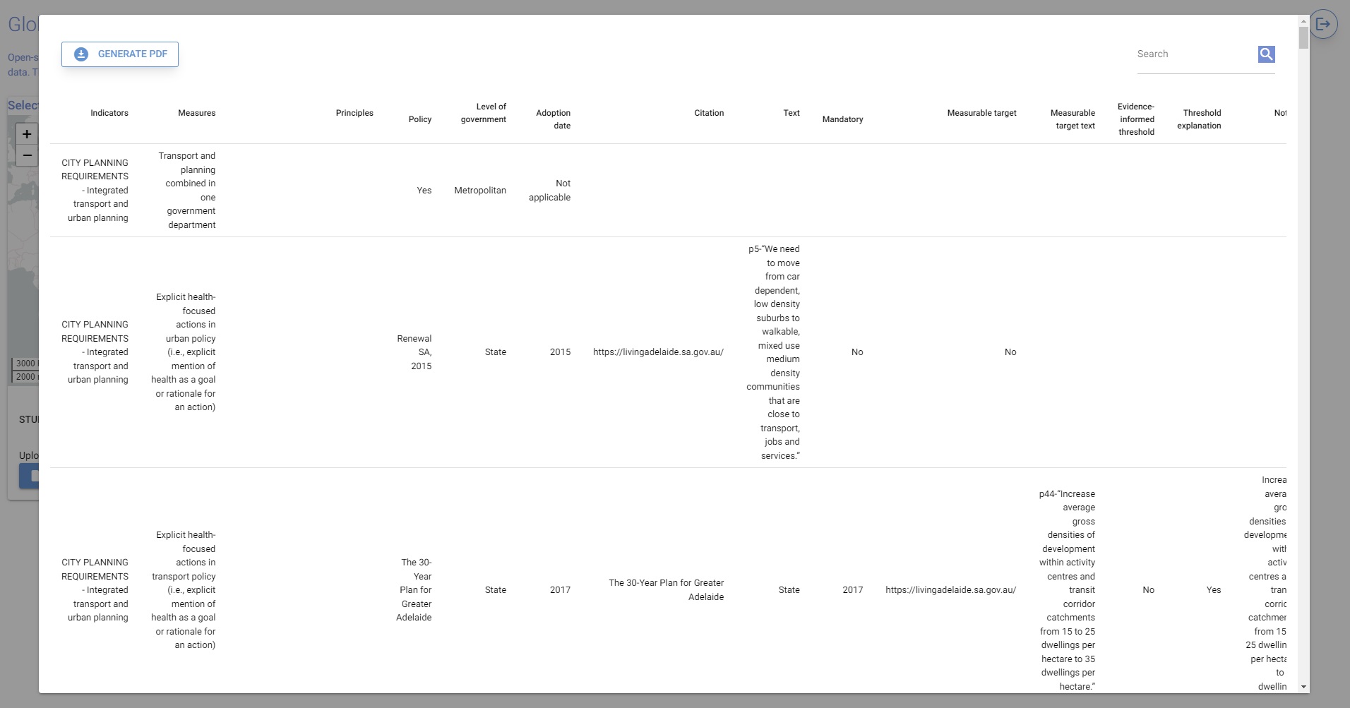
Policy checklist
A policy checklist tool has been developed to support the 1000 Cities Challenge. For more information on the concepts underlying the tool, see: Lowe, M., Adlakha D., et al. (2022). City planning policies to support health and sustainability: an international comparison of policy indicators for 25 cities. The Lancet Global Health, May 2022. https://doi.org/10.1016/S2214-109X(22)00069-9.
Figure 13. Query a completed policy checklist for key phrases, and generate a summary PDF document
An example policy analysis has not yet been provided for Las Palmas. The policy review instrument has recently been updated, and subsequent updates to the software will accommodate this in the reporting templates.
Monitoring progress
Whichever way you choose to use the software, additional output will be displayed that can contain useful information about what is happening following configuration, analysis, generating resources and performing comparisons. When using the web app, you may like to ‘snap’ the terminal window to the left of your screen and your web browser to the right to view both side-by-side.
If anything goes wrong (e.g. you tried to run analysis for a city that hasn’t been fully or correctly configured; see “What if I get stuck“), the process will stop and indicate some kind of error.
Command line usage
As an alternative to running the GHSCI software workflow using the web app as demonstrated in the examples above, or Jupyter Lab, users also have the option to initialise study region configurations, perform analyses, generate resources and comparisons using simple command-line arguments:
Initialise a new study region by entering configure followed by a codename for your study region (e.g. configure example_ES_Las_Palmas_2023). If the command is run without a codename, usage instructions will be displayed. Once a new study region has been initialised, you will be directed to open the newly generated study region configuration file in a text editor and complete details for your city.
For now, we can proceed with analysis for the example city, Las Palmas de Gran Canaria using the provided example. We refer to cities using codenames to avoid ambiguity when identifying study regions. For example, you may want to analyse Las Palmas in both 2023 as well as 2024; or you may be interested in Valencia in Venezuela (e.g. VE_Valencia_2023) as well as Valencia in Spain (ES_Valencia_2023). For Las Palmas, we use the codename example_ES_Las_Palmas_2023.
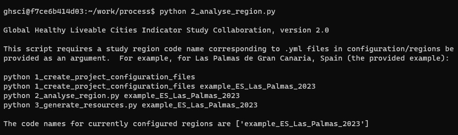
To see the list of codenames for configured cities (Figure 14), enter the commands configure, analysis or generate without providing a codename. For more detailed help on these commands, enter help.
Figure 14. The codenames for configured cities can be viewed by running analysis.
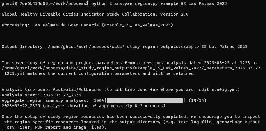
An analysis can now be performed (Figure 15), drawing on the study region configuration file that summarises locations and details for the data that you have retrieved and stored in the data subfolders. For our example city, enter, analysis example_ES_Las_Palmas_2023.
Figure 15. Running neighbourhood analysis for Las Palmas by entering analysis example_ES_Las_Palmas_2023.py.
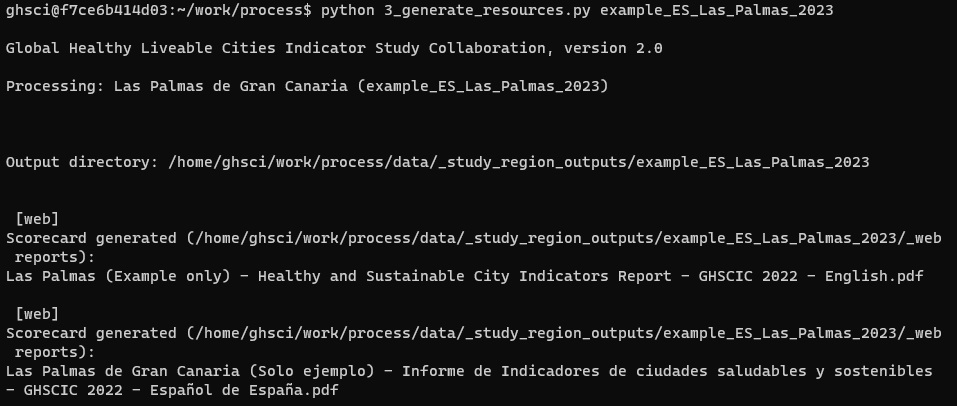
Resources including maps, figures and reports can be generated by entering generate example_ES_Las_Palmas_2023 (or the codename for another city, once you source its data, initialise and complete its configuration, and complete the analysis process; Figure 16).
Figure 16. The output of successful report generation for Las Palmas, which also provides the path to find the output PDF file(s).
Details
Additional general information on configuration, analysis, reporting and comparison steps using the GHSCI software is provided below, including guidance on what to do if you get stuck.
Configuration
Study regions
Before commencing analysis, your study regions will need to be configured with details of your downloaded data, the metadata used to document this data, and parameters to guide the software’s usage of this data in analyses.
The configuration files are text files using the YAML (.yml) format. They can be opened and modified using a text editor to define region specific details, including which datasets are being used, where they were sourced from, and how they should be interpreted. Region configuration files are located within the configuration/regions sub-folder. An example region configuration for Las Palmas de Gran Canaria (for which data supporting analysis is included) has been provided in the file process/configuration/regions/example_ES_Las_Palmas_2023.yml. This can also be viewed online here. At the top of the configuration file are some instructions that describe how to understand and modify the file.
New regions can be added by using the configuration utility functions described elsewhere that initialise a new region configuration file using a city codename at process/configuration/regions/_codename_.yml. This file can be edited using a text editor, or within Jupyter Lab.
Study region template
Click to view description of region configuration parameters
###########################################################
## Study region configuration template v5.0.0 (3 Apri 2024)

## This configuration file uses the YAML format (https://yaml.org/) to describe the data sources, parameters and metadata used to analyse and generate urban indicator resources using the Global Healthy and Sustainable City Indicators software (https://global-healthy-liveable-cities.github.io/).

## Text begining with a double hash symbol ("##") is are comments (used to provide descriptions of how to complete the item immediately below).  Text beginning with a single has symbol ("#") are commented out section of code that may optionally be uncommented as per the provided instructions.

## Optional sections that contain parameters which may be uncommented are marked with a series of hash symbols ("###########") at their start and end lines.

## If entering or modifying a parameter
## - leave a space after the semi-colon
## - indents (ie. 4 spaces) signify a nested sub-list of configurable parameters

## It is recomemnded to view or edit this file in an application providing syntax highlighting, for example, the provided Jupyter Lab web app:
## - type 'lab' at the GHSCI prompt
## - navigate to the "process/configuration/region/" folder in the browser pane
## - double click on the YAML configuration file with name ending in .yml you wish to edit
###########################################################

## Full study region name, e.g. Las Palmas de Gran Canaria
name:
## Target year for analysis, e.g. 2023
year:
## Fully country name, e.g. España
country:
## Two character country code (ISO3166 Alpha-2 code), e.g. ES
country_code:
## Continent name, e.g. Europe
continent:
## Projected coordinate reference system (CRS) metadata
crs:
    ## name of the projected (i.e. units in metres) coordinate reference system (CRS), e.g. REGCAN95 / LAEA Europe
    name:
    ## acronym of the standard catalogue defining this CRS, eg. EPSG
    standard:
    ## Projected CRS spatial reference identifier (SRID) integer that identifies this CRS according to the specified standard, e.g. 5635 (see https://spatialreference.org/, or search for what is commonly used in your city or country; e.g. a national CRS like those listed at https://en.wikipedia.org/wiki/List_of_national_coordinate_reference_systems )
    srid:
## Study region boundary metadata
study_region_boundary:
    ## Path to downloaded data relative to project data directory, or urban_query:variable='value')
    ## e.g. to load a file (geojson, shp, geopackage):
    ## "region_boundaries/Example/Las Palmas de Gran Canaria - Centro Nacional de Información Geográfica - WGS84 - EPSG4326.geojson"
    ## e.g. to use the urban region and urban query specified elsewhere in this configuration file:
    ## urban_query
    ## e.g. to query an attribute for a specific layer in a geopackage
    ## region_boundaries/your_geopackage.gpkg:layer_name -where "some_attribute=='some_value'"
    ## e.g. to query an attribute for a specific layer in a shapefile
    ## region_boundaries/your_shapefile.shp -where "some_attribute=='some_value'"
    data:
    ## The name of the provider of this data, e.g. Centro Nacional de Información Geográfica
    source:
    ## Publication date for study region area data source, or date of currency, e.g. 2019-02-01
    publication_date:
    ## URL for the source dataset, or its provider, e.g. https://datos.gob.es/en/catalogo/e00125901-spaignllm
    url:
    ## Licence for the data, e.g. CC-BY-4.0
    licence:
    ## Whether the provided study region boundary will be further restricted to an urban area defined by its intersection with a linked urban region dataset (see urban_region), e.g. true
    ghsl_urban_intersection: false
    ## A formal citation for this data, For example, "Instituto Geográfico Nacional (2019). Base de datos de divisiones administrativas de España. https://datos.gob.es/en/catalogo/e00125901-spaignllm."
    citation:
    ## Optional notes of relevance for understanding this study region's context
    notes:
###########
## Optional custom aggregation to additional areas of interest (e.g. neighbourhoods, suburbs, specific developments); uncomment and complete to use
# custom_aggregations:
    ## Name for this aggregation layer
    ## The name is followed by a colon, indicating that a list of detail follows
    # custom_layer_using_population_grid:
        ## path to data relative to project data folder
        # data:
        ## The field used as a unique identifier
        # id: 'Codigo'
        ## A list of column field names to be retained
        # keep_columns: Denominaci, cod_postal
        ## The indicator layer to be aggregated ("point" or "grid")
        ## Aggregation is based on the average of intersecting results
        ## unless the agg_distance parameter is defined (see alternative example below)
        # aggregation_source: grid
        ## The variable used for weighting (e.g. 'pop_est' for population when using the grid; leave blank or "false" if using sample points)
        # weight: pop_est
        ## An optional note to provide details about what this aggregation represents
        # note: "Example of aggregating indicators for high school catchment districts within Las Palmas, using the intersection with the population grid and taking the population weighted average of indicators.  Boundary data was derived from data sourced from the open data portal of the Gobierno de Canarias under CC BY 4.0 licence terms: https://opendata.sitcan.es/dataset/centros-educativos/resource/ea650255-c6ea-48c1-84e8-547735624017 (last updated 31 May 2023)."
    ## an example for aggregating for buildings represented in OpenStreetMap
    # buildings_osm_30m:
        # data: "OSM:building is not NULL"
        # keep_columns: building
        ## Distance within metres to use for taking average when aggregating
        ## (see note)
        # aggregate_within_distance: 30
        # aggregation_source: point
        # note: "Example of aggregating using buildings extracted from the configured OpenStreetMap data, taking the average of sample point estimates taken along the pedestrian network within 30m.  This has been done because the point indicators were sampled along the pedestrian network and are therefore unlikely to intersect with buildings.  By taking the average of points within some reasonable distance, the result is like a moving window average that should provide a reasonable representation of the immediate neighbourhood milieu surrounding the building."
## Population metadata (raster or vector)
population:
    ## name of the population data
    name: "Global Human Settlements population data: 2020, Mollweide (EU JRC, 2022)"
    ## path relative to project data directory to folder containing tifs, or to vector file
    data_dir:
    ## type of data (e.g. "raster:Int64" or "vector");  e.g. for GHSL-POP, raster:Int64
    data_type:
    ###########
    ## Vector data specific-fields; uncomment if using vector data (e.g. shp, geojson, gpkg)
    ## The column field with population estimates for your population group of interest (may be total, or for a sub-group of interest to be the focus of your indicators)
    # vector_population_data_field:
    ## The field with the total population data within that area (if you are interested in total, should be the same value as vector_population_data_field)
    # population_denominator:
    ###########
    ###########
    ## Raster data specific-fields; comment out if using raster data (i.e. tif)
    ## image resolution;  e.g. for GHSL-POP with 100 metre resolution, 100m
    resolution:
    ## the image band containing the relevant data, e.g. for GHSL-POP, 1
    raster_band:
    ## A value in the image that represents 'no data', e.g. for GHSL-POP, -200
    raster_nodata:
    ###########
    ## Sample points intersecting grid cells with estimated population less than this will be excluded from analysis.  Depending on your population data resolution, you can use this to exclude areas with very low population due to the uncertainty of where anyone might live in that area, or if they do at all.  For example, 1
    pop_min_threshold:
    ## Coordinate reference system metadata for population data.
    ## For example, for GHSL-POP (Mollweide, ESRI, 54009), enter Mollweide
    crs_name:
    ## For example, for GHSL-POP (Mollweide, ESRI, 54009), enter ESRI
    crs_standard:
    ## For example, for GHSL-POP (Mollweide, ESRI, 54009), enter 54009
    crs_srid:
    ## URL for where this data was sourced from
    source_url:
    ## metadata for citation
    ## when it was published (yyyy), e.g. 2023
    year_published:
    ## the year it is intended to represent (yyyy), e.g. 2020
    year_target:
    ## when you retrieved it (yyyymmdd).  This can be useful to record as data can be subject to revision.  e.g. 20230627
    date_acquired:
    ## licence, e.g. "CC BY 4.0"
    licence: CC BY 4.0
    ## citation, e.g. "Schiavina, M; Freire, S; Carioli, A., MacManus, K (2023): GHS-POP R2023A - GHS population grid multitemporal (1975-2030). European Commission, Joint Research Centre (JRC) [Dataset] doi: 10.2905/D6D86A90-4351-4508-99C1-CB074B022C4A"
    citation:
## OpenStreetMap metadata
OpenStreetMap:
    ## path relative to the project data directory
    data_dir:
    ## the source of the OpenStreetMap data (e.g. Planet OSM, GeoFabrik or OpenStreetMap.fr)
    source:
    ## when it was published (yyyymmdd), e.g. 20230627
    publication_date:
    ## licence (which is most likely ODbL for OpenStreetMap data published since 2012)
    licence: ODbL
    ## the URL from where it was downloaded
    url:
    ## An optional note regarding this data
    note:
## Network analysis related configuration parameters
network:
    #########
    ## Optional network parameters for use in some contexts (eg. island cities)
    ## Whether to only retain main connected network when retrieving OSM roads (set to "false"; the default, which is appropriate for most settings); or retain network 'islands' if present ("true")
    # osmnx_retain_all: false
    ## Whether to extract the network for the buffered study region. It is recommended to set to 'true' (the default) in most cases.  Setting this to false may be appropriate for true islands, but could be problematic for anywhere else where the network and associated amenities may be accessible beyond the edge of the study region boundary).
    # buffered_region: true
    ## Iterate over and combine polygons (this may be appropriate for a series of islands, like Hong Kong), but in most cases it is recommended to be set as false
    # polygon_iteration: false
    ## Minimum total network distance for subgraphs to retain.  This is a useful parameter for customising analysis for islands, like Hong Kong, but for most purposes you can leave this blank (the default).
    # connection_threshold:
    #########
    ## Tolerance in metres for cleaning intersections.  If not providing your own data for evaluating intersection density (see below), this is an important methodological choice.  The chosen parameter should be robust to a variety of network topologies in the city being studied.  See https://github.com/gboeing/osmnx-examples/blob/main/notebooks/04-simplify-graph-consolidate-nodes.ipynb. For example, 12
    intersection_tolerance:
    #########
    ## Optionally, data for evaluating intersections can be provided as an alternative to deriving intersections from OpenStreetMap (where available, this may be preferable); uncomment and complete the required fields to do this.
    ## Custom intersection data settings
    # intersections:
        ## path to data relative to the project data directory
        # data: network_data/your_intersection_data.geojson
        ## citation for optional custom intersection data
        # citation: 'Provider of your intersection data.  YYYY.  Name of your intersection data. https://source-url-for-your-data.place'
        ## a note to describe custom intersection data
        # note: 'Uncomment this configuration section to optionally specify an external dataset of intersections.  Otherwise, these are derived using OpenStreetMap and OSMnx using the intersection_tolerance parameter.  If providing intersection data, you can modify this note for it to be included in the metadata, or remove it.
        #########
## Urban region metadata.   An urban region can optionally be defined to supplement the study region definition, e.g. using the Global Human Settlements Layer Urban Centres Database
urban_region:
    ## name for the urban region data, e.g. "Global Human Settlements urban centres: 2015 (EU JRC, 2019)"
    name:
    ## path to data relative to the project data directory, e.g. "urban_regions/GHS_STAT_UCDB2015MT_GLOBE_R2019A_V1_2.gpkg"
    ## Please note, this data has note been provided but can be retrieved. See the citation below.
    data_dir:
    ## licence, e.g. CC BY 4.0
    licence:
    ## citation for this data, this has been pre-filled for the GHSL UCDB (2019), but change as required if using
    ## For example, for GHSL UCDB (r2019a), enter: "Florczyk, A. et al. (2019): GHS Urban Centre Database 2015, multitemporal and multidimensional attributes, R2019A. European Commission, Joint Research Centre (JRC). https://data.jrc.ec.europa.eu/dataset/53473144-b88c-44bc-b4a3-4583ed1f547e"
    citation:
    ## A list of additional covariates that can be optionally linked for cities included in the GHSL UCDB
    covariates:
        E_EC2E_T15:
            Units: tonnes per annum
            Unit description: tonnes per annum
            Description: Total emission of CO 2 from the transport sector, using non-short-cycle-organic fuels in 2015
        E_EC2O_T15:
            Units: tonnes per annum
            Unit description: tonnes per annum
            Description: Total emission of CO 2 from the energy sector, using short-cycle-organic fuels in 2015
        E_EPM2_T15:
            Units: tonnes per annum
            Unit description: tonnes per annum
            Description: Total emission of PM 2.5 from the transport sector in 2015
        E_CPM2_T14:
            Units: µg per cubic metre
            Unit description: micrograms per cubic meter
            Description: Total concertation of PM 2.5 for reference epoch 2014
        EL_AV_ALS:
            Units: metres above sea level
            Unit description: metres above sea level
            Description: The average elevation estimated within the spatial domain of the Urban Centre, and expressed in metres above sea level (MASL) (EORC & JAXA, 2017).
        E_KG_NM_LST:
            Units: List of climate classes
            Unit description: List of climate classes
            Description: Semi-colon separated list of names of Köppen-Geiger climate classes, intersecting with the spatial domain of the Urban Centre (1986-2010) (Rubel et al., 2017).
        E_WR_T_14:
            Units: °C
            Unit description: Average temperature in Celsius degrees (°C)
            Description: Average temperature calculated from annual average estimates for time interval centred on the year 2015 (the interval spans from 2012 to 2015) within the spatial domain of the Urban Centre, and expressed in Celsius degrees (°C) (Harris et al., 2014).
        E_WR_P_14:
            Units: mm
            Unit description: The amount of rain per square meter in one hour (mm)
            Description: Average precipitations calculated from annual average estimates for time interval centred on the year 2015 (the interval spans from 2012 to 2015) within the spatial domain of the Urban Centre; and expressed in millimetres (mm), the amount of rain per square meter in one hour) (Harris et al., 2014).
## Query used to identify the specific urban region relevant for this region in the Urban Centres database
## GHS or other linkage of covariate data (GHS:variable='value', or path:variable='value' for a dataset with equivalently named fields defined in project parameters for air_pollution_covariates), e.g. GHS:UC_NM_MN=='Las Palmas de Gran Canaria' and CTR_MN_NM=='Spain'
urban_query:
## Additional study region summary covariates to be optionally linked. This is designed to retrieve the list of covariates specifies in the 'urban_region' configuration, either from the configured Global Human Settlements Layer data (enter "urban_query"), or from a CSV file (provide a path relative to the project data directory)
covariate_data:
## Country-level income metadata for additional city context
country_gdp:
    ## Country GDP classification, e.g. lower-middle
    classification:
    ## Citation for the GDP classification, e.g. The World Bank. 2020. World Bank country and lending groups. https://datahelpdesk.worldbank.org/knowledgebase/articles/906519-world-bank-country-and-lending-groups
    citation:
## Details of custom destinations to use (e.g. as done for Maiduguri, Nigeria), in addition to those from OSM (optional, as required; else, leave blank) file name (located in study region folder), category plain name field, category full name field, Y coordinate, X coordinate, EPSG number, attribution
#########
## Optional custom destinations to import in addition to those from (e.g. as done for Maiduguri, Nigeria).  Uncomment if required.
# custom_destinations:
    ## name of file relative to project data directory
    # file:
    ## destination identifier/name
    # name_field:
    ## destination detailed name or description
    # description_field:
    ## y coordinate
    # lat:
    ## x coordinate
    # lon:
    ## EPSG code
    # epsg:
    ## a citation for this data
    # citation:
    #########
#########
## Optional set up for General Transit Feed Specification (GTFS) transit data.
## GTFS feed data is used to evaluate access to public transport stops with regular weekday daytime service
## For cities with no GTFS feeds identified, this may be left commented out.
#gtfs_feeds:
    ## City-specific parent folder in the 'process/data/transit_feeds' directory
    # folder:
    ## list of zipped GTFS feeds saved in above folder
    # name_of_your_gtfs_zip_file.zip:
        ## Name of agency that published this data
        # gtfs_provider:
        ## Year the data was published
        # gtfs_year:
        ## Source URL for the data
        # gtfs_url:
        ## The start date of a representative period for analysis
        ## (outside school holidays and extreme weather events), e.g. Spring/Summer
        ## for Northern Hemisphere: 20230405
        ## for Southern Hemisphere: 20231008
        # start_date_mmdd:
        ## The start date of a representative period for analysis
        ## (outside school holidays and extreme weather events), e.g. Spring/Summer
        ## for Northern Hemisphere: 20230605
        ## for Southern Hemisphere: 20231205
        # end_date_mmdd:
        ## If departure_times within the stop_times.txt file are missing for stops, analysis will be inaccurate unless these are filled in.
        ## In such a case, processing of the GTFS feed will halt with a warning advising the user.
        ## A user could: source alternate data, or fill/interpolate these values themselves.
        ## A function has been provided to perform a linear interpolation according to the provided stop sequence start and end times within each trip_id.
        ## This is an approximation based on the available information, and results may still differ from the actual service frequencies at these stops.
        ## It is the user's responsibility to determine if this interpolation is appropriate for their use case.
        ## To interpolate stop_times where these are missing, set the following parameter to 'true':
        # interpolate_stop_times: false
        ## Optionally the default modes presented here can be modified
        # modes:
            # Tram       : {'route_types': [ 0],'agency_id': }
            # Metro      : {'route_types': [ 1],'agency_id': }
            # Rail       : {'route_types': [ 2],'agency_id': }
            # Bus        : {'route_types': [ 3],'agency_id': }
            # Ferry      : {'route_types': [ 4],'agency_id': }
            # Cable tram : {'route_types': [ 5],'agency_id': }
            # Aerial lift: {'route_types': [ 6],'agency_id': }
            # Funicular  : {'route_types': [ 7],'agency_id': }
            # Trolleybus : {'route_types': [11],'agency_id': }
            # Monorail   : {'route_types': [12],'agency_id': }
            #########
## Optional path to results of policy indicator review for inclusion in generated reports
## See https://healthysustainablecities.github.io/software/#Policy-checklist-data
# e.g. for the example file: process/data/policy_review/Urban policy checklist_1000 Cities Challenge_version 1.0.1_LPGC_Sept23_AQ_JMG - draft example.xlsx
policy_review:
## Optional additional notes for this region
notes:
#########
## Reporting configuration (uncomment to modify)
# reporting:
    ## PDF report templates (uncomment as requires)
    ## Policy templates require completion and configuration of policy review checklist
    # templates:
        # - spatial
        ## - policy_spatial
        ## - policy
    ## Set 'publication_ready' to True once you have checked results, updated the summary and are ready to publish; before then, it should be False.
    # publication_ready: False
    ## Select a basemap for the study region report - options are 'satellite' (recent cloudless composite image of Sentinel-2 satellite imagery to view the urban fabric, https://s2maps.eu by EOX IT Services GmbH), or 'osm' (a light coloured thematic map based on OpenStreetMap with labels), or 'streets' (a light coloured thematic map based on OpenStreetMap without labels, displaying streets),
    # study_region_context_basemap: 'satellite'
    ## Once ready for publication it is recommended to register a DOI for your report, e.g. through figshare, zenodo or other repository
    # doi:
    ## Feature inspiring healthy, sustainable urban design from your city, crediting the source
    # images:
        # 1: # (.jpg, 2100px by 1000px; or 21:10 equivalent aspect ratio)
            # file: "Example image of a vibrant, walkable, urban neighbourhood - landscape.jpg"
            # description: "Example image of a vibrant, walkable, urban neighbourhood with diverse people using active modes of transport and a tram (replace with a photograph, customised in region configuration)"
            # credit: "Feature inspiring healthy, sustainable urban design from your city, crediting the source, e.g.: Carl Higgs, Bing Image Creator, 2023"
        # 2: (.jpg, 2100px by 1000px; or equivalent 21:10 aspect ratio)
            # file: "Example image 2-Landscape.jpg"
            # description: "Example image of a vibrant, walkable, urban area (replace with a photograph or your own image, customised in region configuration)"
            # credit: "Feature inspiring healthy, sustainable urban design from your city, crediting the source, e.g.: Eugen Resendiz, Bing Image Creator, 2023"
        # 3: # (.jpg, 1000px by 1000px; or equivalent 1:1 aspect ratio)
            # file: Example image of a vibrant, walkable, urban neighbourhood - square.jpg
            # description: Example image of a vibrant, walkable, urban neighbourhood with diverse people using active modes of transport and a tram (replace with a photograph, customised in region configuration)
            # credit: "Use your image & credit: e.g. Carl Higgs, Bing Image Creator, 2023"
        # 4: # (.jpg, 1000px by 1000px; or equivalent 1:1 aspect ratio)
            # file: "Example image of climate resilient lively city watercolor-Square.jpg"
            # description: "Example image of a climate-resilient, lively city (replace with an image for your city, customised in region configuration)"
            # credit: "Feature inspiring healthy, sustainable urban design from your city, crediting the source, e.g.: Eugen Resendiz, Bing Image Creator, 2023"
    ## Languages configuration
    # languages:
        ## Add a list of languages as required.  Languages listed should correspond to columns in the _report_configuration.xlsx file 'languages' worksheet.  New languages can be added, although some may require additional fonts.  Some languages may not be supported (eg. complex scripts like Tamil and Thai may not be supported by the report template and require manual edits).
        # English:
            # ## City name in English, for example: Las Palmas
            # name:
            # ## Country name in English, for example: Spain
            # country:
            # ## After reviewing the results, update this summary text to contextualise your findings, and relate to external text and documents (e.g. using website hyperlinks).  This text will be used in the report summary.
            # summary: |
                # After reviewing results for your city, provide a contextualised summary by modifying the "summary" text for each configured language within the region configuration file.
            # ## Contextual summary for study region spatial report.  Users may choose to translate these entries (following the hyphen) for languages configured for their city.  Remember, if you put a colon (":") in, put quotes around the text to make it explicitly understood as text.
            # context:
                # # A brief summary of region characteristics
                # - City context:
                    # # Contextual information about your study region.   Please briefly summarise the city location, history and topography, as relevant.
                    # - summary: Edit the region configuration file to provide background context for your study region. Please briefly summarise the location, history and topography, as relevant.
                    # - source: Add any citations used here.
                # - Levels of government:
                # # For example, for this report, policies from [insert levels of government from policy checklist,  e.g. national, metropolitan, local] levels of government were analysed.Completed policy checklist values will be added, but prose may be customised here.
                    # - summary:
                    # - source: Add any citations used here.
                # - Demographics and health equity:
                    # # For example, highlight socio-economic demographic characteristics and key health challenges and inequities present in this urban area.
                    # - summary:
                    # - source: Add any citations used here.
                # - Environmental disaster context:
                    # # For example, environmental hazards likely to be experience by the urban area over the next 5-10 years, may include [insert those listed as ‘yes’ in the policy checklist].  Completed policy checklist values will be added, but prose may be customised here.
                    # - summary:
                    # - source: Add any citations used here.
    ## Optionally, exceptions to the template can be specified here, this can be useful for additional translation customisation without modifying the report_configuration.xlsx file.  These phrases can incorporate translated phrases defined in report configuration, by enclosing these in curly braces, e.g. like {this}, if 'this' has been defined as a phrase in the relevant language.  See the example region for a demonstration of how this can be used.  Sections from the example can be pasted here and modified as required, or the below example can be uncommented.
    # exceptions:
        # "English":
            # 'author_names': 'Add your names here, or modify authors in config.yml and remove this line'
            # 'policy_jurisdiction': 'Customise the entry for policy jurisdiction to override the record found in a completed policy review checklist.'
        # "Another configured language":
            # 'author_names': 'Agregue sus nombres aquí, o modifique los autores en config.yml y elimine esta línea'
            # 'citation_doi': '{author_names}. 2022. {title_city} — {title_series_line1} {disclaimer} ({city}, {country} — Healthy and Sustainable City Indicators Report: Comparisons with 25 cities internationally. {language} {translation}: {translation_names}). {city_doi}'
#########
Example configuration for Las Palmas de Gran Canaria (Spain) in 2023
Click to view example completion of a record in this file for Las Palmas de Gran Canaria, Spain, using the codename `example_ES_Las_Palmas_2023`.
###########################################################
## Example configuration for Las Palmas de Gran Canaria, Spain
## using Study region configuration template v4.2.2 (27 June 2023)

## This configuration file uses the YAML format (https://yaml.org/) to describe the data sources, parameters and metadata used to analyse and generate urban indicator resources using the Global Healthy and Sustainable City Indicators software (https://healthysustainablecities.github.io/).

## Text begining with a double hash symbol ("##") is are comments (used to provide descriptions of how to complete the item immediately below).  Text beginning with a single has symbol ("#") are commented out section of code that may optionally be uncommented as per the provided instructions.

## Optional sections that contain parameters which may be uncommented are marked with a series of hash symbols ("###########") at their start and end lines.

## It is recomemnded to view or edit this file in an application providing syntax highlighting, for example, the provided Jupyter Lab web app:
## - type 'lab' at the GHSCI prompt
## - navigate to the "process/configuration/region/" folder in the browser pane
## - double click on the YAML configuration file with name ending in .yml you wish to edit
###########################################################

## Full study region name, e.g. Las Palmas de Gran Canaria
name: Las Palmas de Gran Canaria
## Target year for analysis, e.g. 2023
year: 2023
## Fully country name, e.g. España
country: Spain
## Two character country code (ISO3166 Alpha-2 code), e.g. ES
country_code: ES
## Continent name, e.g. Europe
continent: Europe
## coordinate reference system (CRS) metadata
crs:
    ## name of the coordinate reference system (CRS), e.g. REGCAN95 / LAEA Europe
    name: REGCAN95 / LAEA Europe
    ## acronym of the standard catalogue defining this CRS, eg. EPSG
    standard: EPSG
    ## spatial reference identifier (SRID) integer that identifies this CRS according to the specified standard, e.g. 5635 (see https://spatialreference.org/, or search for what is commonly used in your city or country; e.g. a national CRS like those listed at https://en.wikipedia.org/wiki/List_of_national_coordinate_reference_systems )
    srid: 5635
## Study region boundary metadata
study_region_boundary:
    ## Path to downloaded data relative to project data directory, or urban_query:variable='value')
    ## e.g. to load a file (geojson, shp, geopackage):
    ## "region_boundaries/Example/Las Palmas de Gran Canaria - Centro Nacional de Información Geográfica - WGS84 - EPSG4326.geojson"
    ## e.g. to use the urban region and urban query specified elsewhere in this configuration file:
    ## urban_query
    ## e.g. to query an attribute for a specific layer in a geopackage
    ## region_boundaries/your_geopackage.gpkg:layer_name -where some_attribute=="some_value" ## to
    data: "region_boundaries/Example/Las Palmas de Gran Canaria - Centro Nacional de Información Geográfica - WGS84 - EPSG4326.geojson"
    ## The name of the provider of this data, e.g. Centro Nacional de Información Geográfica
    source: Centro Nacional de Información Geográfica
    ## Publication date for study region area data source, or date of currency, e.g. 2019-02-01
    publication_date: 2019-02-01
    ## URL for the source dataset, or its provider, e.g. https://datos.gob.es/en/catalogo/e00125901-spaignllm
    url: https://datos.gob.es/en/catalogo/e00125901-spaignllm
    ## Licence for the data, e.g. CC-BY-4.0
    licence: CC-BY-4.0
    ## Whether the provided study region boundary will be further restricted to an urban area defined by its intersection with a linked urban region dataset (see urban_region), e.g. true
    ghsl_urban_intersection: true
    ## A formal citation for this data, For example, "Instituto Geográfico Nacional (2019). Base de datos de divisiones administrativas de España. https://datos.gob.es/en/catalogo/e00125901-spaignllm."
    citation: "Instituto Geográfico Nacional (2019). Base de datos de divisiones administrativas de España. https://datos.gob.es/en/catalogo/e00125901-spaignllm."
    ## Optional notes of relevance for understanding this study region's context
    notes: manually extracted municipal boundary for Las Palmas de Gran Canaria in WGS84 from the downloaded zip file 'lineas_limite.zip' using QGIS to a geojson file for demonstration purposes."
###########
## Optional custom aggregation to additional areas of interest (e.g. neighbourhoods, suburbs, specific developments); uncomment and complete to use
custom_aggregations:
    ## Name for this aggregation layer
    ## The name is followed by a colon, indicating that a list of detail follows
    school_districts_grid_pop:
        ## path to data relative to project data folder
        data: "region_boundaries/Example/Las Palmas excerpt- gobcan_educacion_areainfluenciacentrosecundaria.geojson"
        ## The field used as a unique identifier
        id: 'Codigo'
        ## A list of column field names to be retained
        keep_columns: Denominaci, cod_postal
        ## The indicator layer to be aggregated ("point" or "grid")
        ## Aggregation is based on the average of intersecting results
        ## unless the agg_distance parameter is defined (see alternative example below)
        aggregation_source: grid
        ## The variable used for weighting (e.g. 'pop_est' for population when using the grid; leave blank or "false" if using sample points)
        weight: pop_est
        note: "Example of aggregating indicators for high school catchment districts within Las Palmas, using the intersection with the population grid and taking the population weighted average of indicators.  Boundary data was derived from data sourced from the open data portal of the Gobierno de Canarias under CC BY 4.0 licence terms: https://opendata.sitcan.es/dataset/centros-educativos/resource/ea650255-c6ea-48c1-84e8-547735624017 (last updated 31 May 2023)."
    ## an example for aggregating for buildings represented in OpenStreetMap
    buildings_osm_30m:
        data: "OSM:building is not NULL"
        keep_columns: building
        ## Distance within metres to use for taking average when aggregating
        ## (see note)
        aggregate_within_distance: 30
        aggregation_source: point
        note: "Example of aggregating using buildings extracted from the configured OpenStreetMap data, taking the average of sample point estimates taken along the pedestrian network within 30m.  This has been done because the point indicators were sampled along the pedestrian network and are therefore unlikely to intersect with buildings.  By taking the average of points within some reasonable distance, the result is like a moving window average that should provide a reasonable representation of the immediate neighbourhood milieu surrounding the building."
###########
## Population metadata (raster or vector)
population:
    ## name of the population data
    name: "Global Human Settlements population data: 2020, Mollweide (EU JRC, 2022)"
    ## path relative to project data directory to folder contining tifs, or to vector file
    data_dir: population_grids/Example/GHS_POP_E2020_GLOBE_R2022A_54009_100_V1_0_R6_C17
    ## type of data (e.g. "raster:Int64" or "vector")
    data_type: raster:Int64
    ###########
    ## Vector data specific-fields; uncomment if using vector data (e.g. shp, geojson, gpkg)
    ## The column field with population estimates for your population group of interest (may be total, or for a sub-group of interest to be the focus of your indicators)
    # vector_population_data_field:
    ## The field with the total population data within that area (if you are interested in total, should be the same value as vector_population_data_field)
    # population_denominator:
    ###########
    ###########
    ## Raster data specific-fields; comment out if using raster data (i.e. tif)
    ## image resolution, e.g. 100 m
    resolution: 100m
    ## the image band containing the relevant data, e.g. for GHSL-POP, 1
    raster_band: 1
    ## A value in the image that represents 'no data', e.g. for GHSL-POP, -200
    raster_nodata: -200
    ###########
    ## Sample points intersecting grid cells with estimated population less than this will be excluded from analysis.  Depending on your population data resolution, you can use this to exclude areas with very low population due to the uncertainty of where anyone might live in that area, or if they do at all
    pop_min_threshold: 1
    ## Coordinate reference system metadata for population data (e.g. Mollweide, ESRI, 54009)
    crs_name: Mollweide
    crs_standard: ESRI
    crs_srid: 54009
    ## URL for where this data was sourced from
    source_url: https://jeodpp.jrc.ec.europa.eu/ftp/jrc-opendata/GHSL/GHS_POP_GLOBE_R2022A/GHS_POP_E2020_GLOBE_R2022A_54009_100/V1-0/tiles/GHS_POP_E2020_GLOBE_R2022A_54009_100_V1_0_R6_C17.zip
    ## metadata for citation
    ## when it was published (yyyy), e.g. 2023
    year_published: 2022
    ## the year it is intended to represent (yyyy), e.g. 2020
    year_target: 2020
    ## when you retrieved it (yyyymmdd).  This can be useful to record as data can be subject to revision.  e.g. 20230627
    date_acquired: 20230222
    ## licence, e.g. "CC BY 4.0"
    licence: CC BY 4.0
    ## citation, e.g. "Schiavina, M; Freire, S; Carioli, A., MacManus, K (2023): GHS-POP R2023A - GHS population grid multitemporal (1975-2030). European Commission, Joint Research Centre (JRC) [Dataset] doi: 10.2905/D6D86A90-4351-4508-99C1-CB074B022C4A"
    citation: "Schiavina, Marcello; Freire, Sergio; MacManus, Kytt (2022): GHS-POP R2022A - GHS population grid multitemporal (1975-2030). European Commission, Joint Research Centre (JRC) [Dataset] doi: 10.2905/D6D86A90-4351-4508-99C1-CB074B022C4A"
## OpenStreetMap metadata
OpenStreetMap:
    ## path relative to the project data directory
    data_dir: OpenStreetMap/Example/example_las_palmas_2023_osm_20230221.pbf
    ## the source of the OpenStreetMap data (e.g. Planet OSM, GeoFabrik or OpenStreetMap.fr)
    source: OpenStreetMap.fr
    ## when it was published (yyyymmdd), e.g. 20230627
    publication_date: 20230221
    ## licence (which is most likely ODbL for OpenStreetMap data published since 2012)
    licence: ODbL
    ## the URL from where it was downloaded
    url: https://download.openstreetmap.fr/extracts/africa/spain/canarias/las_palmas-latest.osm.pbf
    ## An optional note regarding this data
    note: This is configured with a derived excerpt from the larger OpenStreetMap dataset for Las Canarias based on the 1600m buffered municipal boundary of Las Palmas de Gran Canaria to reduce file size for demonstration purposes.
## Network analysis related configuration parameters
network:
    #########
    ## Optional network parameters for use in some contexts (eg. island cities)
    ## Whether to only retain main connected network when retrieving OSM roads (set to "false"; the default, which is appropriate for most settings); or retain network 'islands' if present ("true")
    # osmnx_retain_all: false
    ## Whether to extract the network for the buffered study region. It is recommended to set to 'true' (the default) in most cases.  Setting this to false may be appropriate for true islands, but could be problematic for anywhere else where the network and associated amenities may be accessible beyond the edge of the study region boundary).
    # buffered_region: true
    ## Iterate over and combine polygons (this may be appropriate for a series of islands, like Hong Kong), but in most cases it is recommended to be set as false
    # polygon_iteration: false
    ## Minimum total network distance for subgraphs to retain.  This is a useful parameter for customising analysis for islands, like Hong Kong, but for most purposes you can leave this blank (the default).
    # connection_threshold:
    #########
    ## Tolerance in metres for cleaning intersections.  If not providing your own data for evaluating intersection density (see below), this is an important methodological choice.  The chosen parameter should be robust to a variety of network topologies in the city being studied.  See https://github.com/gboeing/osmnx-examples/blob/main/notebooks/04-simplify-graph-consolidate-nodes.ipynb. For example, 12
    intersection_tolerance: 12
    #########
    ## Optionally, data for evaluating intersections can be provided as an alternative to deriving intersections from OpenStreetMap (where available, this may be preferable); uncomment and complete the required fields to do this.
    ## Custom intersection data settings
    # intersections:
        ## path to data relative to the project data directory
        # data: network_data/your_intersection_data.geojson
        ## citation for optional custom intersection data
        # citation: 'Provider of your intersection data.  YYYY.  Name of your intersection data. https://source-url-for-your-data.place'
        ## a note to describe custom intersection data
        # note: 'Uncomment this configuration section to optionally specify an external dataset of intersections.  Otherwise, these are derived using OpenStreetMap and OSMnx using the intersection_tolerance parameter.  If providing intersection data, you can modify this note for it to be included in the metadata, or remove it.
        #########
## Urban region metadata.   An urban region can optionally be defined to supplement the study region definition, e.g. using the Global Human Settlements Layer Urban Centres Database
urban_region:
    ## name for the urban region data, e.g. "Global Human Settlements urban centres: 2015 (EU JRC, 2019)"
    name: "Global Human Settlements urban centres: 2015 (EU JRC, 2019; Las Palmas de Gran Canaria only)"
    ## path to data relative to the project data directory, e.g. "urban_regions/GHS_STAT_UCDB2015MT_GLOBE_R2019A_V1_2.gpkg"
    ## Please note, this data has note been provided but can be retrieved. See the citation below.
    data_dir: "urban_regions/Example/Las Palmas de Gran Canaria - GHS_STAT_UCDB2015MT_GLOBE_R2019A_V1_2.gpkg"
    ## licence, e.g. CC BY 4.0
    licence: CC BY 4.0
    ## citation for this data, this has been pre-filled for the GHSL UCDB (2019), but change as required if using
    citation: "Florczyk, A. et al. (2019): GHS Urban Centre Database 2015, multitemporal and multidimensional attributes, R2019A. European Commission, Joint Research Centre (JRC). https://data.jrc.ec.europa.eu/dataset/53473144-b88c-44bc-b4a3-4583ed1f547e"
    ## A list of additional covariates that can be optionally linked for cities included in the GHSL UCDB
    covariates:
        E_EC2E_T15:
            Units: tonnes per annum
            Unit description: tonnes per annum
            Description: Total emission of CO 2 from the transport sector, using non-short-cycle-organic fuels in 2015
        E_EC2O_T15:
            Units: tonnes per annum
            Unit description: tonnes per annum
            Description: Total emission of CO 2 from the energy sector, using short-cycle-organic fuels in 2015
        E_EPM2_T15:
            Units: tonnes per annum
            Unit description: tonnes per annum
            Description: Total emission of PM 2.5 from the transport sector in 2015
        E_CPM2_T14:
            Units: µg per cubic metre
            Unit description: micrograms per cubic meter
            Description: Total concertation of PM 2.5 for reference epoch 2014
        EL_AV_ALS:
            Units: metres above sea level
            Unit description: metres above sea level
            Description: The average elevation for the urban centre
        E_KG_NM_LST:
            Units: List of climate classes
            Unit description: List of climate classes
            Description: semi-colon separated list of names of Köppen-Geiger climate classes, intersecting with the spatial domain of the Urban Centre
        E_WR_T_14:
            Units: °C
            Unit description: Average temperature in Celsius degrees (°C)
            Description: average temperature calculated from annual average estimates for time interval centred on the year 1990 (the interval spans from 1988 to 1991) within the spatial domain of the Urban Centre
        E_WR_P_14:
            Units: mm
            Unit description: the amount of rain per square meter in one hour (mm)
            Description: average precipitations calculated from annual average estimates for time interval centred on the year 2015 (the interval spans from 2012 to 2015) within the spatial domain of the Urban Centre
## Query used to identify the specific urban region relevant for this region in the Urban Centres database
## GHS or other linkage of covariate data (GHS:variable='value', or path:variable='value' for a dataset with equivalently named fields defined in project parameters for air_pollution_covariates), e.g. GHS:UC_NM_MN=='Las Palmas de Gran Canaria' and CTR_MN_NM=='Spain'
urban_query: GHS:UC_NM_MN=='Las Palmas de Gran Canaria' and CTR_MN_NM=='Spain'
## Additional study region summary covariates to be optionally linked. This is designed to retrieve the list of covariates specifies in the 'urban_region' configuration, either from the configured Global Human Settlements Layer data (enter "urban_query"), or from a CSV file (provide a path relative to the project data directory)
covariate_data: urban_query
## Country-level income metadata for additional city context
country_gdp:
    ## Country GDP classification, e.g. lower-middle
    classification: High-income
    ## Citation for the GDP classification, e.g. The World Bank. 2020. World Bank country and lending groups. https://datahelpdesk.worldbank.org/knowledgebase/articles/906519-world-bank-country-and-lending-groups
    citation: The World Bank. 2020. World Bank country and lending groups. https://datahelpdesk.worldbank.org/knowledgebase/articles/906519-world-bank-country-and-lending-groups
#########
## Optional custom destinations to import in addition to those from (e.g. as done for Maiduguri, Nigeria).  Uncomment if required.
# custom_destinations:
    ## name of file relative to project data directory
    # file:
    ## category plain name
    # dest_name:
    ## category full name
    # dest_name_full:
    ## y coordinate
    # lat:
    ## x coordinate
    # lon:
    ## EPSG code
    # epsg:
    ## a citation for this data
    # citation:
    #########
#########
## Optional set up for General Transit Feed Specification (GTFS) transit data.
## GTFS feed data is used to evaluate access to public transport stops with regular weekday daytime service
## For cities with no GTFS feeds identified, this may be left commented out.
gtfs_feeds:
    ## City-specific parent folder in the 'process/data/transit_feeds' directory
    folder: Example
    ## list of zipped GTFS feeds saved in above folder
    gtfs_es_las_palmas_de_gran_canaria_guaguas_20230222.zip:
        ## Name of agency that published this data
        gtfs_provider: Guaguas
        ## Year the data was published
        gtfs_year: 2023
        ## Source URL for the data
        gtfs_url: http://www.guaguas.com/transit/google_transit.zip
        ## The start date of a representative period for analysis
        ## (outside school holidays and extreme weather events), e.g. Spring/Summer
        ## for Northern Hemisphere: 20230405
        ## for Southern Hemisphere: 20231008
        start_date_mmdd: 20230405
        ## The start date of a representative period for analysis
        ## (outside school holidays and extreme weather events), e.g. Spring/Summer
        ## for Northern Hemisphere: 20230605
        ## for Southern Hemisphere: 20231205
        end_date_mmdd: 20230605
## Optional path to results of policy indicator review for inclusion in generated reports.
policy_review: process/data/policy_review/_policy_review_template_v0_TO-BE-UPDATED.xlsx
## Optional additional notes for this region
notes:
#########
## Reporting configuration
reporting:
    ## Set 'publication_ready' to True once you have checked results, updated the summary and are ready to publish; before then, it should be False.
    publication_ready: False
    ## Once ready for publication it is recommended to register a DOI for your report, e.g. through figshare, zenodo or other repository
    doi:
    images:
        ## Store images in the process/configuration/assets folder.
        ## Update file name, description and credit as required.
        1:
            file: Example image of a vibrant, walkable, urban neighbourhood - landscape.jpg
            description: Example image of a vibrant, walkable, urban neighbourhood with diverse people using active modes of transport and a tram (replace with a photograph, customised in region configuration)
            credit: Carl Higgs, Bing Image Creator, 2023
        2:
            file: Example image of a vibrant, walkable, urban neighbourhood - square.jpg
            description: Example image of a vibrant, walkable, urban neighbourhood with diverse people using active modes of transport and a tram (replace with a photograph, customised in region configuration)
            credit: Carl Higgs, Bing Image Creator, 2023
    ## Languages configuration
    languages:
        ## Add a list of languages as required.  Languages listed should correspond to columns in the _report_configuration.xlsx file 'languages' worksheet.  New languages can be added, although some may require additional fonts.  Some languages may not be supported (eg. complex scripts like Tamil and Thai may not be supported by the report template and require manual edits).
        English:
            ## City name in English, for example: Las Palmas
            name: Las Palmas
            ## Country name in English, for example: Spain
            country: Spain
            ## After reviewing the results, update this summary text to contextualise your findings, and relate to external text and documents (e.g. using website hyperlinks).  This text will be used in the report summary.
            summary: |
                After reviewing the results, update this summary text to contextualise your findings, and relate to external text and documents (e.g. using website hyperlinks).
        Spanish - Spain:
            name: Las Palmas de Gran Canaria
            country: España
            summary: |
                Después de revisar los resultados, actualice este texto de resumen para contextualizar sus hallazgos y relacionarlo con textos y documentos externos (por ejemplo, utilizando hipervínculos de sitios web).
        Chinese - Simplified:
            name: 大加那利岛拉斯帕尔马斯
            country: 西班牙
            summary: |
                查看结果后,更新此摘要文本以将您的发现置于上下文中,并与外部文本和文档相关(例如使用网站超链接)。
    ## Optionally, exceptions to the template can be specified here, this can be useful for additional translation customisation without modifying the report_configuration.xlsx file.  These phrases can incorporate translated phrases defined in report configuration, by enclosing these in curly braces, e.g. like {this}, if 'this' has been defined as a phrase in the relevant language.  See the example region for a demonstration of how this can be used.  Sections from the example can be pasted here and modified as required, or the below example can be uncommented.
    exceptions:
        "English":
          'local_collaborators_names': 'Add your names here, or modify authors in config.yml and remove this line'
        "Spanish - Spain":
          'local_collaborators_names': 'Agregue sus nombres aquí, o modifique los autores en config.yml y elimine esta línea'
          'citation_doi': '{local_collaborators_names}. 2022. {title_city} — {title_series_line1} {title_series_line2} ({city}, {country} — Healthy and Sustainable City Indicators Report. Traducción al español (España): {translation_names}). {city_doi}'
        "Chinese - Simplified":
          'local_collaborators_names': '在此处添加您的姓名,或在 config.yml 中修改作者并删除此行'
          'citation_doi': '{local_collaborators_names}. 2022. {title_city} — {title_series_line1} {title_series_line2} ({city}, {country} — Healthy and Sustainable City Indicators Report: Comparisons with 25 cities internationally. {language} {translation}: {translation_names}). {city_doi}'
#########
Codenames
Region configuration files are named using a codename to represent a city when used in processing, for example example_ES_Las_Palmas_2023. This helps to avoid issues with ambiguity when analysing multiple cities across different regions and time points (e.g. cities named Valencia are found in both Spain and Venezuala). In the case of our example city, we have used ‘example’ to provide a clarification about the study region’s purpose, ‘ES’ clarifies that this is a Spanish city, ‘Las_Palmas’ is a common short way of writing the city’s name, and the analysis is designed to target 2023, using data sources that could be reasonably assumed to provide a fair representation for the city at that time point.
Initialising
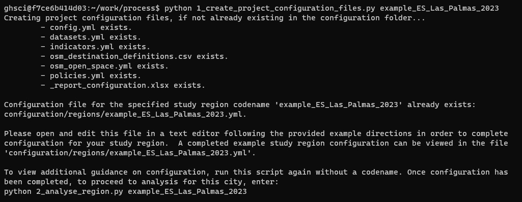
To initialise a new study region configuration file, you can run use the Web app study region form, Jupyter Lab or Python (see example below), or command line (configure <codename>; Figure 17). Running the configuration step for a study region with a previously initialised configuration file (e.g. configure example_ES_Las_Palmas_2023) would advise that the study region configuration has already been initialised, and provide guidance on how to run analyses once configuration has been completed by the user using a text editor.
Figure 17. Output resulting from creating the configuration files; if you were to run this a second time after successfully running it, it would recognise and report that the files already exist, and otherwise remind you about the purpose of the respective configuration files.
Alternatively, you can initialise a configuration file using Python (including using a Jupyter notebook), for example for the Australian city of Melbourne with a target time point of 2023:
1
2
from subprocesses import ghsci
r = ghsci.Region('AU_Melbourne_2023')
Once initialised, study region configuration files must then be modified using a text editor to provide information on the locations of downloaded data and analysis parameters as required.
A good way to view and edit the configuration files is using the provided Jupyter Lab interface.
Other than initialising a new study region (as described above), you can also copy the provided example to a new file and modify the values as required; this might be the easiest way to get started with your new region!
Advanced options
Additional configuration files will be initialised in the process/configuration folder, and may be be edited in a text editor (or in a spreadsheet editor such as Excel for the CSV file) to add and customise analysis for new regions, including
config.yml for overall project configuration, including the names of you, your colleagues and organsisation for inclusion in generated metadata and reports
datasets.yml to optionally define shared datasets and metadata for OpenStreetMap, population, urban regions and transit feeds that can be referenced by multiple study regions
Optionally, projects can be configured to:
analyse GTFS feed data for evaluating accessibility to regularly serviced public transport
use custom sets of OpenStreetMap tags for identifying destinations (see OpenStreetMap TagInfo and region-specific tagging guidelines to inform relevant synonyms for points of interest)
use custom destination data (a path to CSV with coordinates for points of interest for different destination categories can be configured in process/configuration/regions/_codename_.yml)
Configuration file
File description
regions/codename.yml
Used to define and specify details for study regions to be analysed. ** Generate this file by running the configuration script followed by a codename of your choice, then open and edit the resulting text file guided by the provided headings.**
config.yml
Defines general project parameters (e.g. your name and local time zone, for accurate localised recording of start and end times of processing in log files).
osm_open_space.yml
Definitions for identifying areas of open space using OpenStreetMap
datasets.yml
Optionally ysed to define shared datasets and their associated metadata
indicators.yml
Some aspects of indicators calculated can optionally be modified here; currently this is set up for the core indicators of interest for the 1000 City Challenge.
osm_destinations.csv
Used to classify destinations to be retrieved from OpenStreetMap and support calculation of indicators defined in indicators.yml (e.g. percentage of population with access to a particular kind of amenity)
policies.yml
A list of policies for reporting. This is a proof of concept for now, based on the 25-city comparative study. An update is planned to support the new policy template.
Data
When configuring new study region(s), some input data will be required. This is to be stored in sub-folders within the process/data folder. Examples of required data include a population grid, an excerpt from OpenStreetMap, and a study region boundary (either an administrative boundary, or an urban region from the Global Human Settlements Urban Centres Database). Other data are optional: for example, custom boundaries for aggregation (see example), GTFS transit feed data, or a completed policy checklist.
The kinds of data that can be configured for usage are summarised in the below table. We have provided examples for each of these for Las Palmas, with the exception at the time of writing of a completed policy checklist.
Population distribution raster grid or vector data with coverage of urban region of interest. GHS population grid (R2023) is recommended (for example, the 2020 Molleweide 100m grid tiles corresponding to your area of interest, with these saved and extracted to a folder like process/data/GHS/R2023A/GHS_POP_E2020_GLOBE_R2023A_54009_100_V1_0, which may be specified in process/configuration/datasets.yml. Take care to select the correct Epoch for your analysis before downloading!
Conditional
region_boundaries
Vector boundary for identifying study region (e.g. geopackage, geojson or shp). If a geopackage is used, a specific layer can optionally be specified and queried, as per this example
Collections of zipped GTFS feeds to represent public transport service frequency
Optional
other_custom_data
Other custom data, such as points of interest
Specific paths to data are configurable in the configuration files. However, in general, it is recommended that input data be stored within subfolders of the data folder as per the provided example.
OpenStreetMap data
OpenStreetMap data are used to represent features of interest within regions of interest.
This can be retrieved in .pbf (recommended; smaller file size) or .osm format from sites including:
It is recommended that a suffix to indicate publication date is added to the name of downloaded files as a record of the time point at which the excerpt is considered representative of the region of interest e.g. “las_palmas-latest.osm_20230210.pbf” or “oceania_yyyymmdd.pbf” where yyyy is the year, mm is the 2-digit numerical month, and dd is the 2-digit numerical day date_.
The main considerations are that the excerpt is as small as possible while ensuring that it has complete coverage of the region(s) of interest (and about 1600 metres additional beyond the boundary, or as otherwise configured). Using a smaller rather than a larger file will speed up processing.
For example, for a project considering multiple cities in Spain, the researchers could download an excerpt for the country of Spain or for specific sub-regions like Catalunya as required to ensure that the region of interest is encompassed within the extract. Using the example of Spain, which also contains regions outside Europe, if sourcing from Geofabrik as the example links above, it is worth noting that the excerpts are grouped by continent so some care should be taken. For example, Las Palmas de Gran Canaria are found under Canary Islands in Africa on Geofabrik, or a smaller PBF specifically for Las Palmas can be retrieved from download.openstreetmap.fr under ‘africa/spain/canarias’. Our software provides example data for Las Palmas, and to reduce file size we prepared a clipped portion of the data around this city using only the minimum area required..
Population grid data
Population grid or vector data are used to represent the population distribution within regions of interest.
We recommend usage and configuration of the R2023a or more recent population data from the Global Human Settlements Layer project, with a time point of 2020 (or as otherwise appropriate for your project needs, and bearing in mind the limitations of the GHSL population model) and using Mollweide (equal areas, 100m) projection. note: take care when retrieving the GHSL population data to select the correct Epoch! The default at the time of writing is a population projection for 2030, however currently the most relevant dataset are the 2020 estimates; make sure to select 2020
This file is approximately 5 GB in size, so if you are only analysing one or a few cities, it may be worth identifying the specific tiles that relate to your study region(s) using the interactive map downloader provided by GHSL and storing them as suggested above.
The citation for the data is: Schiavina M., Freire S., MacManus K. (2022): GHS-POP R2022A - GHS population grid multitemporal (1975-2030).European Commission, Joint Research Centre (JRC). https://doi.org/10.2905/D6D86A90-4351-4508-99C1-CB074B022C4A
Optionally, official population data can be used if this is judged to be more accurate or meaningful for your city’s analysis and interpretation of results by your intended audience. For example, to use the official 1km Australian population grid for 2021 (instead of the 100m grid estimates from the GHSL-POP r2022a dataset for 2020 or 2025), this could be specified as per the following code block:
1
2
3
4
5
6
7
8
9
10
11
12
13
14
15
16
17
population:
    name: "Australian Population Grid 2021 (ABS, 2023)"
    data_dir: population_grids/Australian_Population_Grid_2021_in_TIFF_format
    data_type: raster:Int64
    resolution: 1km
    raster_band: 1
    raster_nodata:
    pop_min_threshold: 5
    crs_name: GDA94 / Australian Albers
    crs_standard: EPSG
    crs_srid: 3577
    source_url: https://www.abs.gov.au/statistics/people/population/regional-population/2021/GEOTIFF.zip
    year_published: 2022
    year_target: 2021
    date_acquired: 20230302
    licence: CC BY 4.0
    citation: "Australian Bureau of Statistics (2022), Australian Population Grid 2021. https://www.abs.gov.au/statistics/people/population/regional-population/2021"
Optionally, population estimates from a vector data source can also be configured, for example:
population:
    alias: catalunya_2021
    name: "Població de Catalunya georeferenciada a 1 de gener de 2021"
    data_dir: population_grids/gridpoblacio01012021/gridpoblacio_01012021.shp
    vector_population_data_field: TOTAL
    population_denominator: TOTAL
    crs_name: ETRS89 / UTM zone 31N
    crs_standard: ESRI
    crs_srid: 25831
    source_url: https://www.idescat.cat/serveis/biblioteca/docs/bib/publicacions/gridpoblacio01012021.zip
    provider: Institut d’Estadística de Catalunya
    year_published: 2023
    year_target: 2021
    date_acquired: 20230608
    licence: CC BY 4.0
    licence_url: https://creativecommons.org/licenses/by/4.0/deed.ast
    data_type: vector
    pop_min_threshold: 1
    # urban sample points intersecting grid cells with estimated population less than this will be excluded from analysis
    citation: "Població De Catalunya Georeferenciada a 1 De Gener De .. Barcelona: Generalitat de Catalunya. Institut d'Estadística de Catalunya, 2016. https://biblio.idescat.cat/publicacions/Record/21104"
In the above vector data example, this contains multiple fields with estimates by age group which opens up additional possibilities for analysis of indicators for specific population sub-groups (in this case, using age). To do this, one could modify the vector_population_data_field to the field containing the population of interest, e.g.
1
vector_population_data_field: P_15_64
In this way, age-specific indicators could be calculated and compared. Indicators based on overall population density use the estimates from the population_denominator field; hence, if you are interested in overall population for your indicators the data_field and the denominator should share the same value.
Choice of population data grid is an important methodological choice for analysts as it determines the resolution at which results are output (for example a choice between 100m estimated population, or 1000m official population statistic, or administrative areas of varying dimensions). As such, it is good to know that this is an option available to ensure your indicator results serve their intended purpose and audience.
Region boundary data
Region boundary data are used to identify the study region(s) of interest. These may be retrievable from a government open data portal, or the UN OCHA Humanitarian Data Exchange.
Additional custom region boundaries can be used for custom aggregations, as per the example:
###########
## Optional custom aggregation to additional areas of interest (e.g. neighbourhoods, suburbs, specific developments):
custom_aggregations:
    ## Name for this aggregation layer
    ## The name is followed by a colon, indicating that a list of detail follows
    school_districts_grid_pop:
        ## path to data relative to project data folder
        data: "region_boundaries/Example/Las Palmas excerpt- gobcan_educacion_areainfluenciacentrosecundaria.geojson"
        ## The field used as a unique identifier
        id: 'Codigo'
        ## A list of column field names to be retained
        keep_columns: Denominaci, cod_postal
        ## The indicator layer to be aggregated ("point" or "grid")
        ## Aggregation is based on the average of intersecting results
        ## unless the agg_distance parameter is defined (see alternative example below)
        aggregation_source: grid
        ## The variable used for weighting (e.g. 'pop_est' for population when using the grid; leave blank or "false" if using sample points)
        weight: pop_est
        note: "Example of aggregating indicators for high school catchment districts within Las Palmas, using the intersection with the population grid and taking the population weighted average of indicators.  Boundary data was derived from data sourced from the open data portal of the Gobierno de Canarias under CC BY 4.0 licence terms: https://opendata.sitcan.es/dataset/centros-educativos/resource/ea650255-c6ea-48c1-84e8-547735624017 (last updated 31 May 2023)."
    ## an example for aggregating for buildings represented in OpenStreetMap
    buildings_osm_30m:
        data: "OSM:building is not NULL"
        keep_columns: building
        ## Distance within metres to use for taking average when aggregating
        ## (see note)
        aggregate_within_distance: 30
        aggregation_source: point
        note: "Example of aggregating using buildings extracted from the configured OpenStreetMap data, taking the average of sample point estimates taken along the pedestrian network within 30m.  This has been done because the point indicators were sampled along the pedestrian network and are therefore unlikely to intersect with buildings.  By taking the average of points within some reasonable distance, the result is like a moving window average that should provide a reasonable representation of the immediate neighbourhood milieu surrounding the building."
###########
Urban region data
Urban region data are used to optionally identify and restrict analysis to the urban portion of a study region, and optionally can also be used to identify an urban region of interest (e.g. an urban agglomeration surrounding a major city). Additionally, city-level urban covariates contained within the database may be linked with the final estimates (e.g. air pollution estimates).
The dataset linked above represents urban centres in 2015, and may be cited as: Florczyk A., Corbane C,. Schiavina M., Pesaresi M., Maffenini L., Melchiorri, M., Politis P., Sabo F., Freire S., Ehrlich D., Kemper T., Tommasi P., Airaghi D., Zanchetta L. (2019) GHS Urban Centre Database 2015, multitemporal and multidimensional attributes, R2019A. European Commission, Joint Research Centre (JRC)PID: https://data.jrc.ec.europa.eu/dataset/53473144-b88c-44bc-b4a3-4583ed1f547e
Policy checklist data
The global-indicators software has been designed to report on both policy and spatial indicator results. Once the policy checklist has been completed for a city, save this in the project data folder (e.g. within data/policy_review). Using the GHSCI web app interface you can now select this completed file to view, query and generate a PDF summary report.
GTFS transit feed data
Collections of General Transit Feed Specification (GTFS) feeds are used to represent public transport service frequency. See the GTFS reference for details on what is required for GTFS feeds. More than one transit operator may operate in the region of interest, so it is important to aim to have full coverage of both the region and the operators, without overlap of services, to represent the service frequency of public transport stops in a city.
We recommend that zipped feeds be stored in a region specific GTFS parent folder, e.g. “Spain - Valencia”, that contains one or zipped GTFS feeds, e.g. gtfs_spain_valencia_EMT_20190403.zip and gtfs_spain_valencia_MetroValencia_20190403.zip. The parent folder and specific feeds are configured in the region configuration file. For example,
## Optional set up for General Transit Feed Specification (GTFS) transit data.
## GTFS feed data is used to evaluate access to public transport stops with regular weekday daytime service
## For cities with no GTFS feeds identified, this may be left commented out.
gtfs_feeds:
    ## City-specific parent folder in the 'process/data/transit_feeds' directory
    folder: Example
    ## list of zipped GTFS feeds saved in above folder
    gtfs_es_las_palmas_de_gran_canaria_guaguas_20230222.zip:
        ## Name of agency that published this data
        gtfs_provider: Guaguas
        ## Year the data was published
        gtfs_year: 2023
        ## Source URL for the data
        gtfs_url: http://www.guaguas.com/transit/google_transit.zip
        ## The start date of a representative period for analysis
        ## (outside school holidays and extreme weather events), e.g. Spring/Summer
        ## for Northern Hemisphere: 20230405
        ## for Southern Hemisphere: 20231008
        start_date_mmdd: 20230405
        ## The start date of a representative period for analysis
        ## (outside school holidays and extreme weather events), e.g. Spring/Summer
        ## for Northern Hemisphere: 20230605
        ## for Southern Hemisphere: 20231205
        end_date_mmdd: 20230605
Some GTFS feeds don’t adhere to the reference standard and some customisation is possible to accomodate mapping of alternate route_types and agency_id values. The defaults for these fields can be seen in the datasets.yml file here. These can be over-ridden for each mode, for example, for the below feed which describes service schedules for a semi-Metro a route type of 400 was used. This was mapped as a value for the ‘Tram’ mode to allow analysis to progress:
1
2
3
4
5
6
7
8
9
gtfs_feeds:
    folder: Marc issues/Malaga
    20230519_130136_Metro_Malaga:
      gtfs_provider: Metro de Málaga
      gtfs_year: 2023
      start_date_mmdd: 20230519
      end_date_mmdd: 20230831
      modes:
        Tram: {'route_types': [400]}
Multiple values can also be specified, e.g.,
1
2
modes:
  Bus: {'route_types': [700,712,714]}
However, in most cases the route_type values for a feed (found in the routes.txt file) should correspond to the defaults of the specification, in which case the modes parameter can be omitted as per the example configuration. This will draw upon the default settings.
Data output folder
Generated resources are saved to study region specific codename sub-folders within the data/_study_region_outputs directory.
The following provides an indicative list of the contents of this folder (italics indicate a word that will vary depending on configuration):
Item
Type
Description
_web reports
Folder
Contains generated policy and spatial indicator reports, optionally in multiple languages
figures
Folder
Contains generated maps and figures
__region name__codename_processing_log.txt
text file
A text file that is progressively appended to with the screen outputs for analyses that are not otherwise displayed. This contains a record of processing, and is useful when debugging if something has gone awry with a particular configuration or supplied data
_parameters.yml
text file
A text file containing records of the most recent configuration analysed (on detection of a new version, older versions will be retained with a suffix indicating the date at which it was current)
analysis_report_yyyy-mm-dd_hhmm.pdf
PDF file
A PDF report summarising approach taken for analysis of the core set of spatial indicators and generation of associated resources
A CSV spreadsheet containing a comparison of summary indicator results for a reference study region and a comparison study region (generated as a result of running the compare process)
codename_1600m_buffer.gpkg
Geopackage file
A geopackage containing derived study region features of interest used in analyses, and including grid and overall summary results for this region
codenameindicators{resolution}_yyyy.csv
CSV file
Grid or small area summary results of indicator analysis for this region
codename_indicators_region.csv
CSV file
Overall summary results of indicator analysis for this region
codename_metadata.xml
XML file
XML metadata (ISO19115)
codename_metadata.yml
YML file
YML metadata
output_data_dictionary.csv
CSV file
CSV data dictionary
output_data_dictionary.xlsx
XLSX file
Formatted Excel data dictionary
codename_osm_yyyymmdd.pbf
PBF file
An excerpt from OpenStreetMap for this buffered study region as configured
poly_codename.poly
text file
A polygon boundary file; this is generated for the buffered urban region of interest as per configuration in regions/codename.yml, and is used to excerpt a portion of OpenStreetMap for this region from the configured input data
A population raster for this buffered study region, excerpted from the input data, in the projects coordinate reference system
population_resolution_codename_source crs.tif
TIF file
A population raster for this buffered study region, excerpted from the input data, in the coordinate reference system of the input population data (e.g. Mollweide, in the case of the recommended GHS-POP data)
Frequently Asked Questions
From June 2024, we are migrating our Frequently Asked Questions and the directions in this website to our GHSCI Wiki where we will maintain an updated list of tips for using the software to analyse and report on urban indicators.
What if I get stuck?
Check the log file
Sometimes things go wrong, and you might get a message advising you of this. For example, an entry in the region configuration YAML might be missing a space after a colon character (for example, :true instead of : true) or a path to data may have a typographical error. The nature of warnings will depend on how you are running the software. However, if your configuration file has successfully been loaded and analysis has commenced, the most informative place to look is the text file log that can be found in the data output folder for your study region. Open this file in a text editor and scroll to the end to find the point where things may have gone awry.
Check configurations
If the data output folder for your study region hasn’t been created or doesn’t contain an analysis text log after attempting to run the analysis workflow, it is likely that an error in your configuration file has prevented it being successfully loaded. Check to see if an error was displayed, e.g. advising that configured data files could not be located at the paths specified. Consider comparing your study region configuration with the provided example and see what might differ. A small error could stop the file being successfully loaded, but in many cases there are clues given as to where to find and correct this.
Configuration files are easier to read and edit in a text editor that provides syntax highlighting. For example, you can view and edit the YAML files using the provided Jupyter Lab interface in your web browser. Alternatively, there are software options such as VS Code or Notepad++.
Check for issues
Other users or the developers themselves may have come across the issue you are experiencing and posted a question or resolution for this on our software code repository. You can browse, query or add a comment to open or closed issues here.
Report a bug, request a feature, or contribute to the project
Perhaps you have come across a use case or data format that we haven’t considered or accounted for. You can report a bug or make a feature request online here. To ensure our community can help you, try to provide as much contextual detail as possible. This can include copying text from your log file and configuration file(s) as appropriate; often the solutions will be found by understanding what is contained in these documents.
Contributions are welcome! Some advice on doing this is found here.
Processing time
The time taken to run analyses will vary depending on city size and density of features, and the specification of the computer running analyses. A minimum of 8GB of RAM is recommended; in general, the more RAM and processors available, the better. It is possible that lower specification machines will be able to perform analyses of smaller urban regions. The provided example city of Las Palmas de Gran Canaria should take about 8 minutes to run on a standard laptop, however some larger cities may take a number of hours to process.
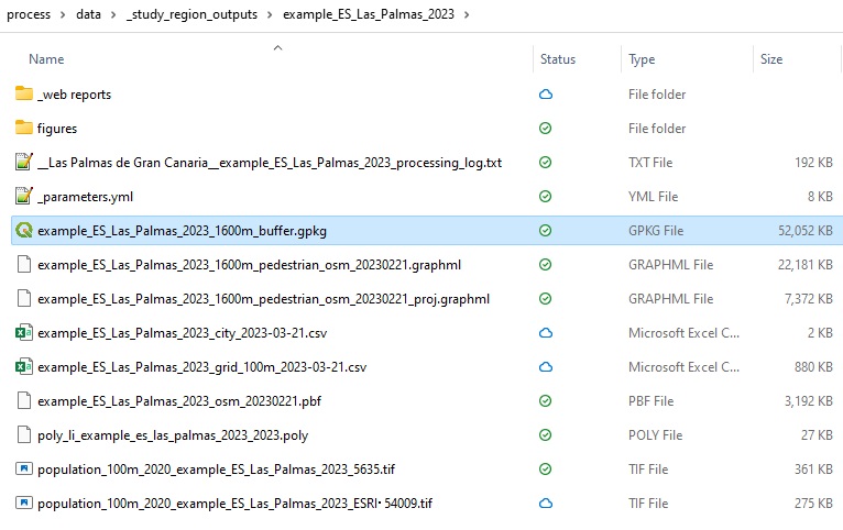
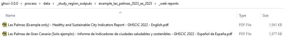
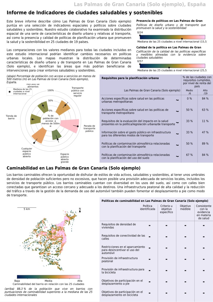
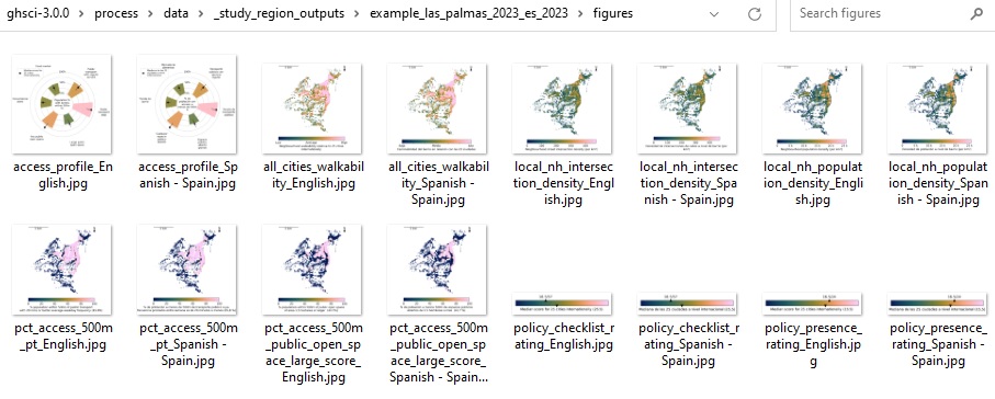
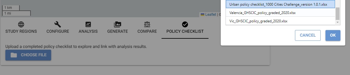 .
.